Building a biological knowledge graph at Pendulum using Amazon Neptune

This is a guest post by Connor Skennerton, Staff Data Engineer at Pendulum Therapeutics.

At Pendulum, we combine state-of-the-art genome sequencing, cell culturing, and manufacturing processes to produce Pendulum Glucose Control, the only medical probiotic clinically shown to lower blood glucose spikes for the dietary management of type 2 diabetes through the gut microbiome. Research and development at Pendulum requires the synthesis of a diverse set of rich data and information streams, and this year we undertook a project to aggregate much of our data into a single database, the Pendulum knowledge graph, which integrates publicly available information on bacterial metabolism with the DNA sequencing data we generate for our strains.

The building blocks of life are compounds, small molecules that do everything from power our cells to build proteins, fats, and carbohydrates, which are constantly being created, converted, and consumed by enzymes. There are thousands of enzymes that produce a complex graph of biochemical reactions. This graph can be decomposed into subsets that we call pathways, which are composed of enzymes working together in a step-by-step fashion to perform large-scale chemical transformations. Biology has a great knack for taking parts of things and reusing them for some other purpose; looking at the butyrate pathway from the Kyoto Encyclopedia of Genes and Genomes (KEGG), there is an astounding amount of branching into variants and other pathways.

Understanding these pathways has been a major topic of biological research for over 70 years. Through it, scientists have amassed a great catalog of metabolic pathways, more of which are being discovered every year. Understanding this information by querying, searching, and analyzing these pathways and their connections can provide amazing insights into how microorganisms live and how they can contribute to a healthy gut.

We represent our knowledge graph as a property graph in Amazon Neptune, a fast, reliable, fully managed graph database service that makes it easy to build and run applications that work with highly connected datasets. We use Neptune as the backend for an API and web-service for our lab and data scientists.

During the development of our knowledge graph, we also considered using a relational SQL database. However, in biology, one-to-many or many-to-many relationships are the norm, not the exception, and this requires additional tables in SQL to be produced to just manage the relationships. Queries in SQL inevitably result in many joins that affect performance, and there is the added burden of strict data modeling, index creation and tuning, and migrating schemas from one version to the next. In contrast, highly connected biological data fits very naturally in a graph database, and the schema-less data model in Neptune made it easy to integrate new information.

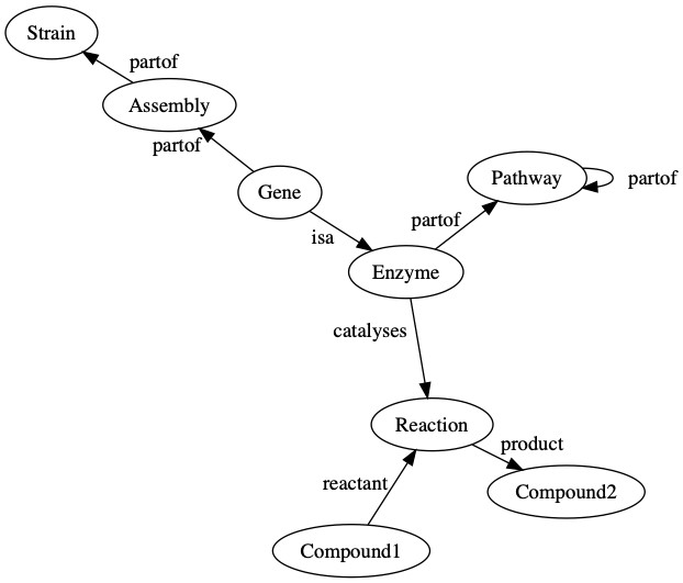
We use a knowledge graph to connect compounds to the biochemical reactions that produce or consume them. These reactions are linked to the enzymes that catalyze these reactions, and we then link the enzymes to the pathways in which they are involved. Enzymes are created from genes that are found on assemblies, which are an observation of the genome of a strain. The following diagram is a general representation of biological data in Pendulum’s knowledge graph.

We chose to model our data in Amazon Neptune using a labeled property graph, where the objects in the graph (the nodes) and the relationships between them (the edges) have attributes (properties). For example, an enzyme node has the property EC number and name, which tells you which specific enzyme it is among all others. In the Pendulum knowledge graph, we have many different node types, including:

• Compounds
• Reactions
• Enzymes
• Pathways
• Genes
• Assemblies
• Strains

Populating our graph is of course crucial and made difficult by the multitude of different file formats from bioinformatics databases. One of the most popular of these resources is KEGG, which has information about biochemical compounds, reactions, enzymes, and metabolic pathways, each of which is defined in a similar (but distinct) record file format. Thankfully, the Biopython project already has text parsers for these file formats, and after parsing the KEGG data, we created a CSV file of all the nodes and edges, and used the fast loader API in Neptune to quickly get data in.

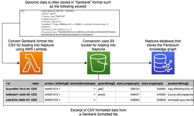
With this backbone loaded, we added genomes and linked their genes to their respective enzymes and metabolic pathways. AWS has a growing library of open access genomic datasets, and many thousands of publicly available genome sequences are available at the National Center for Biotechnology Information’s assembly database in genbank format, which is a record oriented text file format containing information about the genes and all the various metadata associated with them. We use the Biopython library to convert our annotated genomes into the same CSV format for Neptune to ingest. The following diagram is an overview of our genome upload process.

In this post, we use this graph to answer some important biological questions, but first we discuss some basics to familiarize ourselves with querying graph databases. Neptune uses the Gremlin query language (for more information, see Getting Started). In the following example code, I use Python and the gremlinpython package to access the database:

import pandas as pd
from gremlin_python import statics
from gremlin_python.process.anonymous_traversal import traversal
from gremlin_python.process.graph_traversal import __
from gremlin_python.process.strategies import *
from gremlin_python.driver.driver_remote_connection import DriverRemoteConnection
from gremlin_python.process.traversal import T
from gremlin_python.process.traversal import Order
from gremlin_python.process.traversal import Cardinality
from gremlin_python.process.traversal import Column
from gremlin_python.process.traversal import Direction
from gremlin_python.process.traversal import Operator
from gremlin_python.process.traversal import P
from gremlin_python.process.traversal import Pop
from gremlin_python.process.traversal import Scope
from gremlin_python.process.traversal import Barrier
from gremlin_python.process.traversal import Bindings
from gremlin_python.process.traversal import WithOptions

NEPTUNE_ENDPOINT = "<FILL IN YOUR ENDPOINT HERE>"
g = traversal().withRemote(DriverRemoteConnection(NEPTUNE_ENDPOINT,'g'))

The last line in the preceding code creates the graph variable (g). The graph variable is created from a traversal, which is an abstraction around a graph. For more information, see Gremlin’s Anatomy. We want the traversal to be connected to Neptune, which is accomplished by .withRemote(DriverRemoteConnection. This hooks up all the pipes between the Neptune database and our client program.

How much data is in the knowledge graph right now?

The following query groups all the vertices in the graph by their label and counts them:

node_types = g.V().groupCount().by(T.label).next()
pd.DataFrame.from_dict(node_types, orient='index').sort_values(0, ascending=False)

The following table summarizes the count of node types in the database (these values have been fuzzed).

 The query contains the following elements:

• V() – Start with all the vertices (nodes) in the graph.
• .groupCount().by(T.label) – Group all the nodes by their label and count them. Labels are a special property of nodes that defines their type (like CDS or reaction). Labels help with indexing and organizing your data.
• .next() – This final piece is a terminal step, meaning it runs the query and returns the first result. There are a number of terminal steps, and without them your queries don’t actually run.

How many genes are in each pathway for an organism?

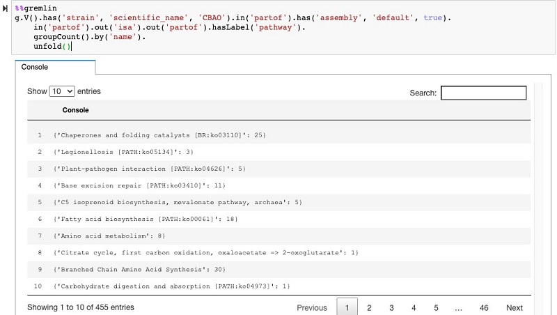
We can see from the grouping that there are a lot of CDS nodes—these are the genes on the genomes. We can use the graph to also find out how many of those genes are in each pathway with the following type of traversal:

# Get a count of the genes in each pathway for this strain
g.V().has('strain', 'scientific_name', 'CBAO').in_('partof').has('assembly', 'default', True).in_('partof').out('isa').out('partof').hasLabel('pathway').groupCount().by('name').unfold()

The code has the following elements:

• V().has(…) – Start at a specific strain
• in_('partof').out('isa').out('partof').hasLabel('pathway') – Walk the graph through the gene nodes, the enzymes, and then to the pathways (refer back to the graph overview to follow this traversal)
• .groupCount().by('name') – Group all the nodes by the pathway name and count them

The following screenshot shows the query in the Neptune workbench and the table output of the traversal results.

Which genes are part of a pathway?

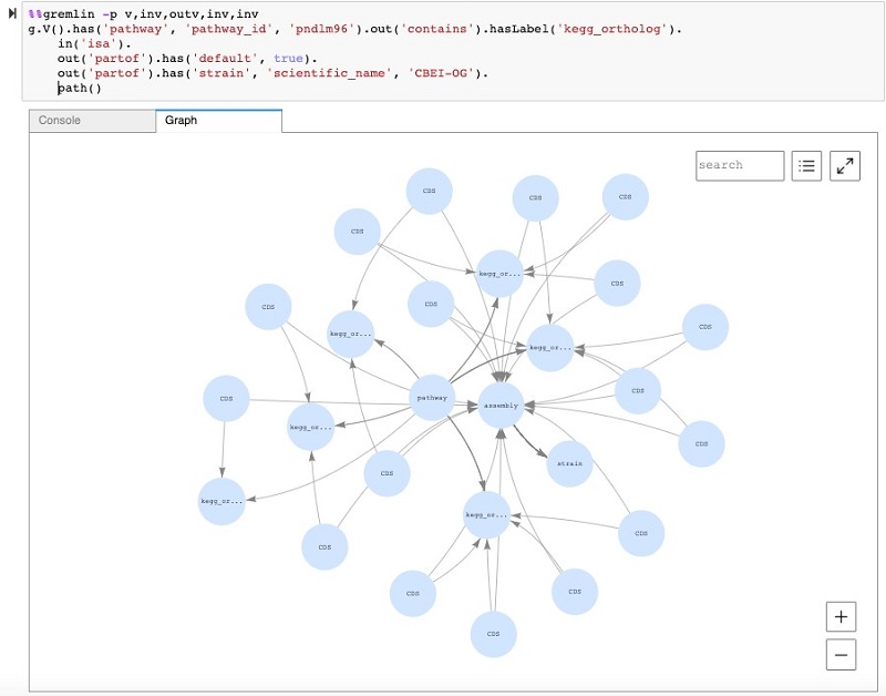
We can take this general query a step further to look at the subgraph that connects a specific pathway to a certain strain. We can further use the Neptune workbench’s visualization capability to see all these connections. In the following screenshot, you can see a query that begins at a specific pathway and traverses to a strain node. In this case, instead of counting the nodes like earlier, we use the path step at the end, which enables the visualization of the subgraph.

What enzymes produce butyrate?

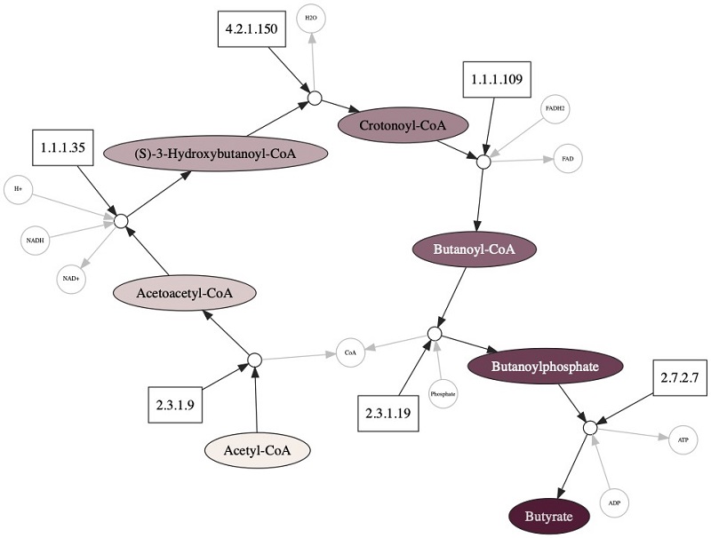
One natural question is to ask which of our genomes can produce or consume certain compounds. For this post, we use butyrate as an example. Butyrate is a key molecule needed for balancing insulin and glucose levels. At Pendulum, we’re especially interested in Butyrate because people with T2D have lost beneficial bacterial strains that produce butyrate. One of the ways that bacteria makes butyrate is from Acetyl-CoA, which requires six enzymes.

The following diagram shows a subset of our knowledge graph, with one pathway that synthesizes butyrate. The primary compounds converted in the pathway are shown in large colored nodes; other compounds that participate are shown in small grey nodes. Enzymes that catalyze these reactions are shown as rectangles, and the reaction nodes are shown as small white circles.

To find the enzymes that use butyrate, we use the following code:

# lets find all the enzymes that use butyrate
uses_butyrate = g.V().has("compound", "name", "Butyrate").both().in_('catalyzes').hasLabel("enzyme").valueMap().toList()

for enzyme in uses_butyrate:
    print(enzyme['EC_number'][0], enzyme['name'][0])

The list contains 2.7.2.7, which we show in the following table with four other enzymes that use butyrate but aren’t related to our pathway of interest.

The query contains the following elements:

• g.V() – Start with all the vertices (nodes) of the graph
• .has("compound", "name", "Butyrate") – Filter so we’re only looking for the nodes that have a compound label and a name property with the value Butyrate
• .both() – Walk from the compound nodes to adjacent nodes; these are the reactions that produce or consume butyrate
• .in_('catalyzes') – Walk from the reaction nodes to adjacent nodes along in edges with a catalyzes label
• .hasLabel("enzyme") – Make sure they are enzyme type node
• We’re now at the enzyme nodes that catalyze the reactions that produce or consume butyrate. We find out the identities of these enzymes by returning a map of all their properties (.valueMap().toList()).

From the preceding query, you can see that we recovered the last step of the butyrate pathway (enzyme 2.7.2.7) but not any of the previous steps because we only walked one iteration from butyrate to the reaction nodes. It’s possible to keep walking though the graph to recover all the reactions.

Which organisms have the most genes in the butyrate production pathway?

An alternative to walking through all the reactions for every query is to associate sets of reactions with a pathway, so if we know the pathway we can walk to the enzymes of interest. An interesting comparison then becomes which organisms contain those sets of enzymes that have been organized into pathways. See the following code:

# small formatting function to turn results into pandas table
def reformat_pathway_count(n):
    data= {}
    for genome, pathways in n.items():
        try:
            data['genome'].append(genome)
        except KeyError:
            data['genome'] = [genome]

        for p, c in pathways.items():
            try:
                data[p].append(c)
            except KeyError:
                data[p] = [c]
    return pd.DataFrame(data).set_index('genome').sort_index()[:5]

# query to get the count of enzymes per pathway per strain
n = g.V().has('pathway', 'kegg_pathway_id', P.within("00650", "00010")).as_('pathway').
     out('partof').hasLabel('enzyme').as_('ortho').
     in_('isa').hasLabel('CDS').as_('gene').
     out('partof').hasLabel('assembly').as_('org').
     group().
       by('md5').
       by(__.group().
            by(__.select('pathway').by('name')).
            by(__.select('ortho').by(T.id).dedup().fold().count(Scope.local))).next()

reformat_pathway_count(n)

The query contains the following elements:

• g.V() – Start with all the vertices (nodes) of the graph.
• has('pathway', 'kegg_pathway_id',P.within("00650", "00010")) – Filter so we’re only looking at the KEGG pathway with the ID 00650 or 00010. In this case, that’s the Butanoate metabolism pathway or Glycolysis.
• out('contains').hasLabel('enzyme') – Walk from the pathway to all the enzymes in that pathway.
• in_('isa').hasLabel('CDS') – Walk along in edges to find all the genes that are annotated to be those enzymes.
• out('partof').hasLabel('assembly') – Walk along to the genome assembly that has those genes.
• group().by('md5').by(__.group() – This is the start of the fancy part—a multi-layered group. We choose the outermost grouping to be the md5 hash of the assembly (this is a property of assembly nodes in Pendulum’s graph), and the values of this grouping are another group.
• by(__.select(‘pathway’).by(‘name’)) – The keys of the inner grouping are the names of the pathways. Here we make use of the select step in Gremlin, which allows us to go back to previous nodes in the traversal (in this case, the pathway nodes at the beginning) to get their values.
• by(__.select('ortho').by(T.id).dedup().fold().count(Scope.local)) – Finally, the values of the inner group—the count of enzymes that belong to that pathway. Again, this starts by selecting previous nodes in the traversal (_ .select('ortho')) and getting their IDs (.by(T.id)). We dereplicate these enzyme nodes (.dedup()) and fold() them into a list of values before finally counting them. The fold step is crucial—try removing it from the query to see what happens.

Conclusion

Graph databases provide an extremely flexible representation for the analysis of highly connected data that we work with in biotechnology. Neptune offers numerous features that simplify adding external data to our knowledge graph. This post showed examples of simple and more complex queries that are of interest to our scientists at Pendulum. Due to the expressiveness of the Gremlin query language, many more possibilities are waiting to be explored. There is a huge amount of potential by linking all this data together!

About the Author

Connor Skennerton, PhD, is a Staff Data Engineer as Pendulum Therapeutics. With a background in microbiology, his goal is to integrate the plethora of information that scientists discover to develop novel treatments for the world’s chronic diseases. In his free time, he enjoys rock climbing and hiking.