As enterprises grow and data and performance needs increase, purpose-built databases have become the new way to tackle specific data access patterns. Modeling and querying highly connected datasets on a traditional relational database can be performance intensive, and expressing relational-style queries against these datasets can be challenging. Graph databases like Amazon Neptune provide a new means for storing and querying highly connected datasets quickly and at massive scale.
To access the insights in your data using this technology, you first need to model the data as a graph. Often, the data exists across the enterprise in existing relational databases. Converting relational data structures to graph models can be complex and involve constructing and managing custom extract, transform, and load (ETL) pipelines. AWS Database Migration Service (AWS DMS) can manage this process efficiently and repeatably, whether you’re migrating a full application to Neptune or only copying a subset of your relational data for graph-specific use cases.
In this four-part series, we cover how to translate a relational data model to a graph data model using a small dataset containing airports and the air routes that connect them. Part one discussed the source data model and the motivation for moving to a graph model. Part two covered designing the property graph model. In this post, we explore mapping our relational data model to a Resource Description Framework (RDF) model. You may wish to refer to parts one and two of the series to review the model. In part four, we show how to use AWS DMS to copy data from a relational database to Neptune for both graph data models.
Designing the RDF Model
An RDF knowledge graph, although built from nodes and edges, is conceptually different from the labeled property graph model we explored in the previous post. All data in the graph is stored as triples—statements consisting of a subject, predicate, and object.
When modeling for RDF, you focus on semantics and model the domain concepts and their meaning in context. Rather than using labels, which are class-like, but informal, we assign types, often using established ontologies to allow for shared understanding of concepts within the graph. In our use case, we look at countries, their airports, and the routes between these airports. When possible, we use the DBpedia ontology to support a shared understanding of resource types.
Each resource representing the row of a particular table has a type based on that table. The resource itself is identified by a unique IRI that can be built using the row’s primary key. Foreign key relationships are modeled with predicate IRIs. Unlike the property graph model, everything is modeled as a triple, and non-foreign key columns are modeled with predicates corresponding to those columns with literal values as the objects. Pure junction tables create triples where the table becomes the predicate connecting subject and object resources corresponding to the foreign keys. Because RDF predicates can’t have associated properties (a predicate IRI can’t be the subject of a different triple), we need a different approach when there is data associated with the edge. We discuss that in the following section.
In the following examples, we use the Turtle serialization of RDF to provide more details.
COUNTRY
The COUNTRY table models countries of the world. We use the DBpedia ontology’s Country class (dbo:Country) as the type of each country instance. We use the primary key COUNTRY_ID to construct the country instance’s IRI. The COUNTRY_CODE column is the ISO 3166-1 two-character code. There’s a dbo: predicate for that relation, which we also use. We use the OFFICIAL_NAME column value as the label, using the standard rdfs:label predicate. The corresponding RDF looks like the following code (the predicate a, read "is a," is shorthand used in Turtle and SPARQL for the RDF predicate rdf:type):
AIRPORT
The AIRPORT table models commercial airports of the world. We use the DBpedia ontology’s Airport class (dbo:Airport) as the type of each airport instance. We use the primary key AIRPORT_ID to construct the airport instance’s IRI. The AIRPORT_CODE column is the IATA location identifier. There’s a dbo: predicate for that relation, which we also use. As with the COUNTRY table, we use the OFFICIAL_NAME column as the label using the rdfs:label predicate.
The foreign key column COUNTRY_ID denotes that the airport exists in that country. There’s a dbo: predicate we can use that models that relationship, dbo:country. The corresponding RDF looks like the following code:
ROUTE
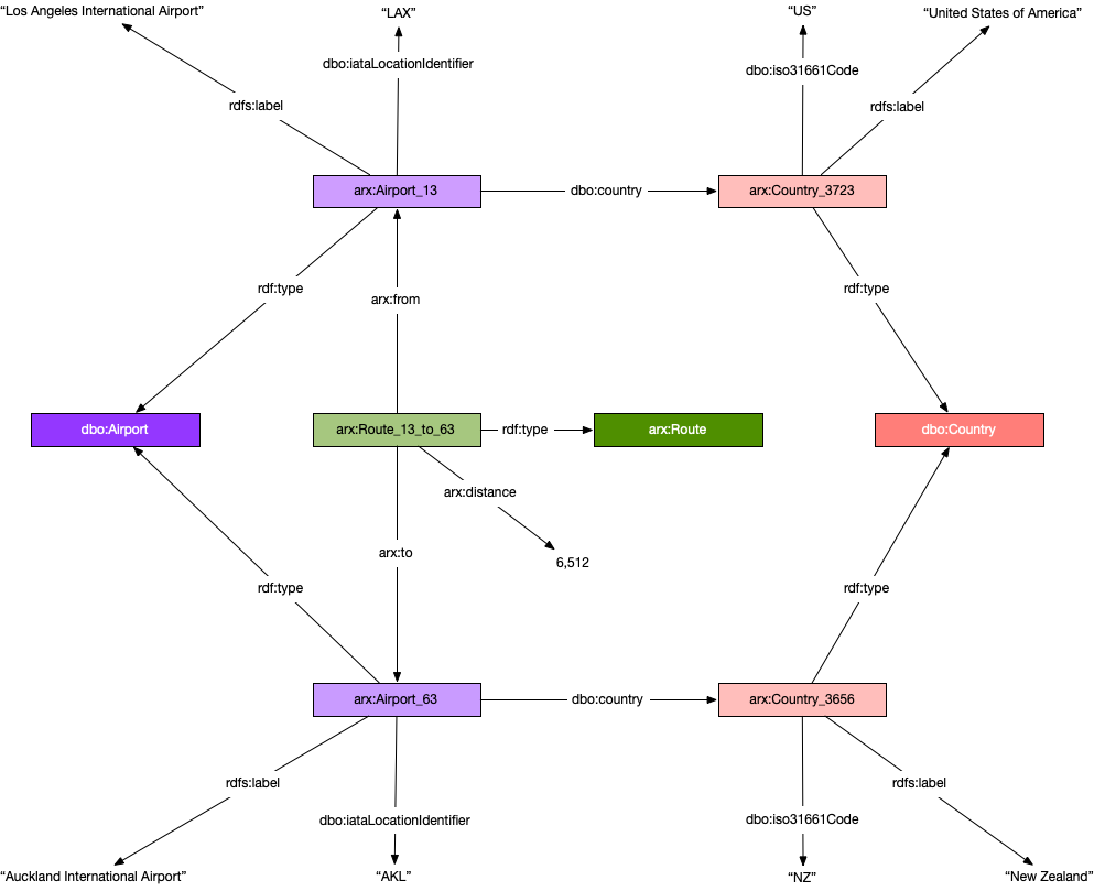
Routes connect two airports and have an associated distance. In the property graph we modeled, this as an edge with distance as an edge property. In RDF, we must take a different approach. There are different ways to model this. For this post, we model the route as a resource with rdf:type route. That route has arx:from and arx:to predicates, and an arx:distance predicate to hold the distance literal. The corresponding RDF looks like the following code:
In the following diagram, you can see the difference from the preceding property graph model. Everything is a triple. Subjects must be resources. All properties are modeled as edges. Object literals associated with predicates such as arx:distance (an integer) and dbo:iataLocationCode (a character string) are leaf nodes in the graph.

Using R2RML to map relational data to an RDF model
RDB to RDF mapping language (R2RML) is a W3C recommendation for describing the mapping from a relational database (RDB) to RDF. AWS DMS tasks use R2RML to guide the migration and translation of a source RDBMS to a Neptune RDF graph. R2RML is expressed using Turtle and consists of a series of triples maps, one for each logical table being migrated. R2RML introduces a specific vocabulary to define the mappings.
AWS DMS supports a subset of R2RM, but doesn’t include inverse expressions, joins, and virtual tables. In the following code, we use templates to create IRIs for object resources.
The following is the R2RML for the COUNTRY table:
In the preceding code, the table mapping is described as an rr:TriplesMap. The rr:TriplesMap has three parts. First, it defines the logical table and specifies the actual table name used in the source database, in this case countries. Next, we define the subject. This is done using rr:subjectMap. The subject map defines the RDFS class of the subject (see the following code):
The IRI is defined using a simple template that references the primary key column of the table:
The part of the string enclosed in curly braces, {COUNTRY_ID}, is replaced by the value of the COUNTRY_ID column (for our use case, New Zealand, the primary key is 3656). The namespace and other structure of the IRI is designed as appropriate for the model being developed.
Each non-primary key column is mapped using a predicate object map, rr:predicateObjectMap. This mapping provides the predicate to use for the column and the actual database column name to reference. By default, the column value is defined as a literal value with an appropriate data type. In this use case, we map the AIRPORT_CODE column to dbo:iataLocationIdentifier, which is a string value.
When a column value is a foreign key reference to another RDBMS table, the object value should be defined as an IRI. In this case, the IRI is generated using a template, just like we used in the rr:subjectMap. An additional triple is added to the rr:objectMap to state that the term is an IRI. This is shown in the following code defining the mapping of the COUNTRY column from the AIRPORT table map to the COUNTRY table:
Interacting with the graphs
Now that the migration is complete, we can interact with the graph. We use Amazon Neptune Workbench to look at both models we created.
RDF graph on Neptune Workbench
We now look at the RDF knowledge graph we built from the same relational source data. Our dataset has 3,497 airports, but no details about the kind of airport. We can easily use the information we just migrated to classify the international airports. First, we define an international airport class with the following code:
Then we insert some new triples to define any airport that has commercial routes to another country as an arx:InternationalAirport:
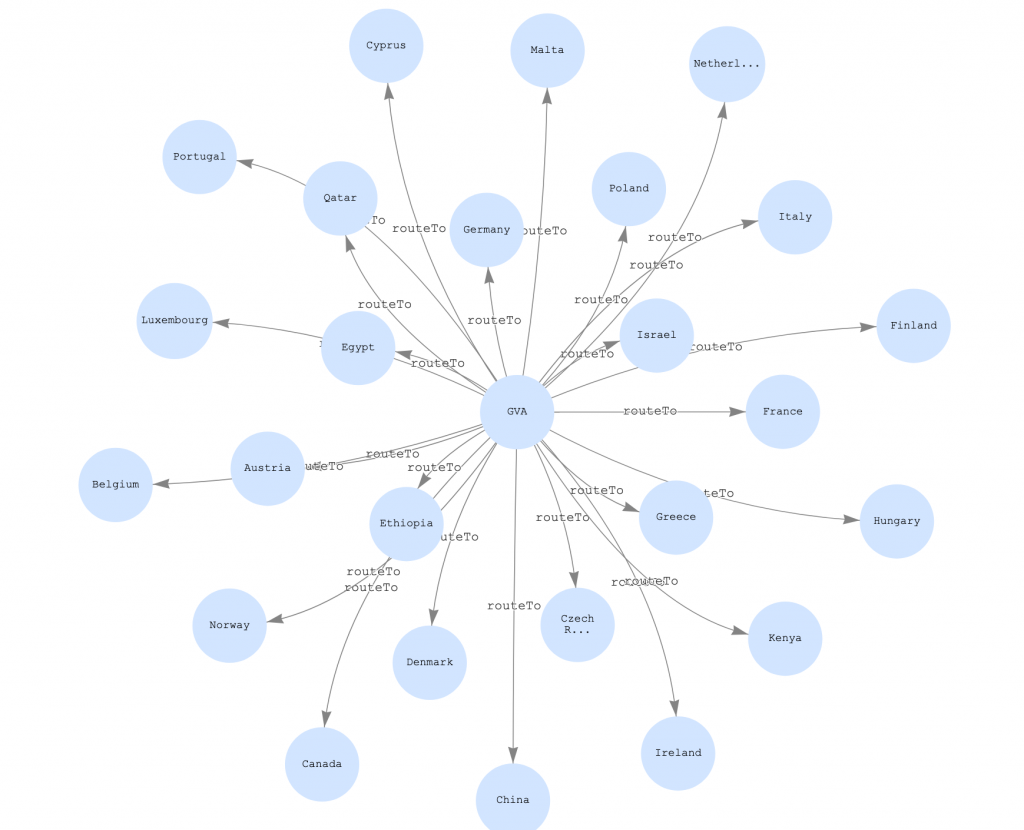
Now we can use the Neptune Workbench visualization feature to visualize some international airports and the countries to which they have flights. The following code shows the query.
The following table contains the first 10 results.
| s | p | o | |
| 1 | GVA | routeTo | Luxembourg |
| 2 | GVA | routeTo | Austria |
| 3 | GVA | routeTo | Belgium |
| 4 | GVA | routeTo | Canada |
| 5 | GVA | routeTo | China |
| 6 | GVA | routeTo | Cyprus |
| 7 | GVA | routeTo | Czech Republic |
| 8 | GVA | routeTo | Denmark |
| 9 | GVA | routeTo | Germany |
| 10 | GVA | routeTo | Egypt |
Then, we use the Neptune Workbench visualization capabilities to show the results.

Finally, our database is all about airports, but it doesn’t have any information on the airlines that use them. These relationships exist in DBpedia, and we can find them using SPARQL 1.1 Federation to align our airport resources with those in DBpedia, and then find the airlines using the dbo:hubAirport relationship. See the following code:
In the query, we align the airport entities using the IATA location identifier and use the dbo:hubAirport relationship to find the associated airlines. The following table shows the five airlines that use Seattle-Tacoma International Airport as a hub.
| 1 | http://air_routes.example.com/ns#Airport_22 | North Pacific Airlines | Seattle–Tacoma International Airport |
| 2 | http://air_routes.example.com/ns#Airport_22 | Alaska Airlines | Seattle–Tacoma International Airport |
| 3 | http://air_routes.example.com/ns#Airport_22 | Delta Connection | Seattle–Tacoma International Airport |
| 4 | http://air_routes.example.com/ns#Airport_22 | Horizon Air | Seattle–Tacoma International Airport |
| 5 | http://air_routes.example.com/ns#Airport_22 | Delta Air Lines | Seattle–Tacoma International Airport |
Summary
This series of posts discusses how to translate a relational data model to a graph data model. In this post, we designed a mapping from our relational data model to an RDF model. We use the R2RML file that defines the mapping in the next and final post of our series.
If you have any questions, comments, or other feedback, share your thoughts on the Amazon Neptune Discussion Forums.
About the author
 Chris Smith is a Principal Solutions Architect on the AWS Database Services Organization Customer Advisory Team focusing on Neptune. He works with customers to solve business problems using Amazon graph technologies. Semantic modeling, knowledge representation, and NLP are subjects of particular interest.
