Populating your graph in Amazon Neptune from a relational database using AWS Database Migration Service (DMS) – Part 2: Designing the property graph model

As enterprises grow and data and performance needs increase, purpose-built databases have become the new way to tackle specific data access patterns. Modeling and querying highly connected datasets on a traditional relational database can be performance intensive, and expressing relational-style queries against these datasets can be challenging. Graph databases like Amazon Neptune provide a new means for storing and querying highly connected datasets quickly and at massive scale.

To access the insights in your data using this technology, you first need to model the data as a graph. Often, the data exists across the enterprise in existing relational databases. Converting relational data structures to graph models can be complex and involve constructing and managing custom extract, transform, and load (ETL) pipelines. AWS Database Migration Service (AWS DMS) can manage this process efficiently and repeatably, whether you’re migrating a full application to Neptune or only copying a subset of your relational data for graph-specific use cases.

In this four-part series, we cover how to translate a relational data model to a graph data model using a small dataset containing airports and the air routes that connect them. Part one discussed the source data model and the motivation for moving to a graph model. In this post, we explore mapping our relational data model to a labeled property graph model. You may wish to refer to part one of the series to review the source relational data model. Part three covers the Resource Description Framework (RDF) data model. In part four, we show how to use AWS DMS to copy data from a relational database to Neptune for both graph data models.

Designing the property graph model

We typically map relational table rows to vertices in a property graph model. Vertices have a label that is generally taken from the relational table name. Vertices also require a vertex ID, and we use the row’s primary key to create the ID.

Foreign key relationships are modeled as edges in the property graph model. Edges have a label that may be derived from the foreign key column name. Edges also require an edge ID, which we can construct from the primary and foreign key values.

Columns that aren’t foreign keys are modeled as properties—key-value pairs where the key is the column name and the value is the column value. Junction tables—tables whose primary purpose is to model one-to-many or many-to-many relations—have to be modeled a bit differently. Rows in a junction table are modeled as edges. Additional columns become properties on the edge.

In this section, we use our example relational database to expand further on these concepts.

COUNTRY

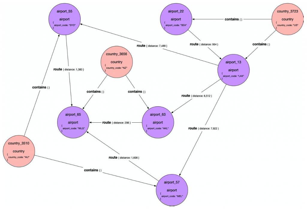
New Zealand is in the COUNTRY table of our relational database. The primary key, COUNTRY_ID, is 3656. The OFFICIAL_NAME column value is New Zealand, and the two-character COUNTRY_CODE column value is NZ.

This row is modeled as a vertex. The label of the vertex is country and the vertex ID is country_3656, using the row’s primary key. We use the OFFICIAL_NAME and COUNTRY_CODE columns to create properties on the vertex.

AIRPORT

Wellington International Airport is found in our relational model with the primary key column AIRPORT_ID equal to 65. The OFFICIAL_NAME column value is Wellington International Airport, and the IATA AIRPORT_CODE column value is WLG. We use these two columns to create properties on the vertex. The AIRPORT table also has a foreign key column COUNTRY_ID equal to 3656, which relates the airport to its country, in this case New Zealand. This becomes an edge.

Because there is a primary key and a foreign key, this row creates both a vertex and an edge. The label of the vertex is airport and the vertex ID is airport_65, using the primary key. The edge represents the fact that the airport is in the identified country.

Edges in a property graph have direction—the edge connects from one vertex to the other vertex. When creating the edge, you have to decide which direction the edge should go to support the traversals you intend to use and to label the edge appropriately. For our use case, we want to look at connections between countries via their airports, so a contains relationship works well. That means we create a contains edge from country_3656 to airport_65. Edges require a unique edge ID, so we construct that using the primary keys of the COUNTRY row and the AIRPORT row: c3656_contains_a65.

ROUTE

The ROUTE table resembles a junction table. It has two foreign key columns, FROM_AIRPORT_ID and TO_AIRPORT_ID, and the integer column DISTANCE_IN_MILES. Each row defines a route between two airports. This is modeled as an edge. The direction of the edge is naturally from-to. The DISTANCE_IN_MILES value becomes a property on the edge. We use the first row of our example table to create an edge from Seattle-Tacoma International Airport to Los Angeles International Airport. The edge label is route and the edge ID is a22_route_a13. An edge property, distance, is set to 954.

Visually, a portion of the graph looks like the following diagram.

Graph mapping configuration file

Finally, AWS DMS defines a JSON format, called a graph mapping configuration file, to specify these mappings and drive the migration. It consists of an array of rules that define the desired transformations.

In each rule, you specify the source relational table name and then describe one or more vertex definitions. The format is easy to follow. The template key-value lines are important to understand. Keys such as vertex_id_template, property_value_template, or edge_id_template can substitute values from the relational database table columns. For example, when encountering “vertex_id_template”: “airport_{AIRPORT_ID}”, AWS DMS substitutes the value from the AIRPORT_ID column to create a vertex ID of, for example, airport_13. The following code shows a portion of the configuration file:

{ 
    "rules": [ 
        { 
            "rule_id": "1", 
            "rule_name": "vertex_mapping_rule_from_airport", 
            "table_name": "AIRPORT", 
            "vertex_definitions": [ 
                { 
                    "vertex_id_template": "airport_{AIRPORT_ID}", 
                    "vertex_label": "airport", 
                    "vertex_definition_id": "1", 
                    "vertex_properties": [ 
                    ] 
                } 
            ] 
        }, 
        … 
        { 
            "rule_id": "3", 
            "rule_name": "edge_mapping_rule_from_route", 
            "table_name": "ROUTE", 
            "edge_definitions": [ 
                { 
                    "from_vertex": 
                    { 
                        "vertex_id_template": "airport_{FROM_AIRPORT_ID}", 
                        "vertex_definition_id": "1" 
                    }, 
                    "to_vertex": 
                    { 
                        "vertex_id_template": "airport_{TO_AIRPORT_ID}", 
                        "vertex_definition_id": "1" 
                    }, 
                    "edge_id_template": 
                    { 
                        "label": "route", 
                        "template" : "a{FROM_AIRPORT_ID}_route_a{TO_AIRPORT_ID}" 
                    }, 
                    "edge_properties":[ 
                        { 
                            "property_name": "distance", 
                            "property_value_template": "{DISTANCE_IN_MILES}", 
                            "property_value_type": "int" 
                        } 
                    ] 
                } 
            ] 
        }, 
        … 
    ] 
} 

Property graph on Neptune Workbench

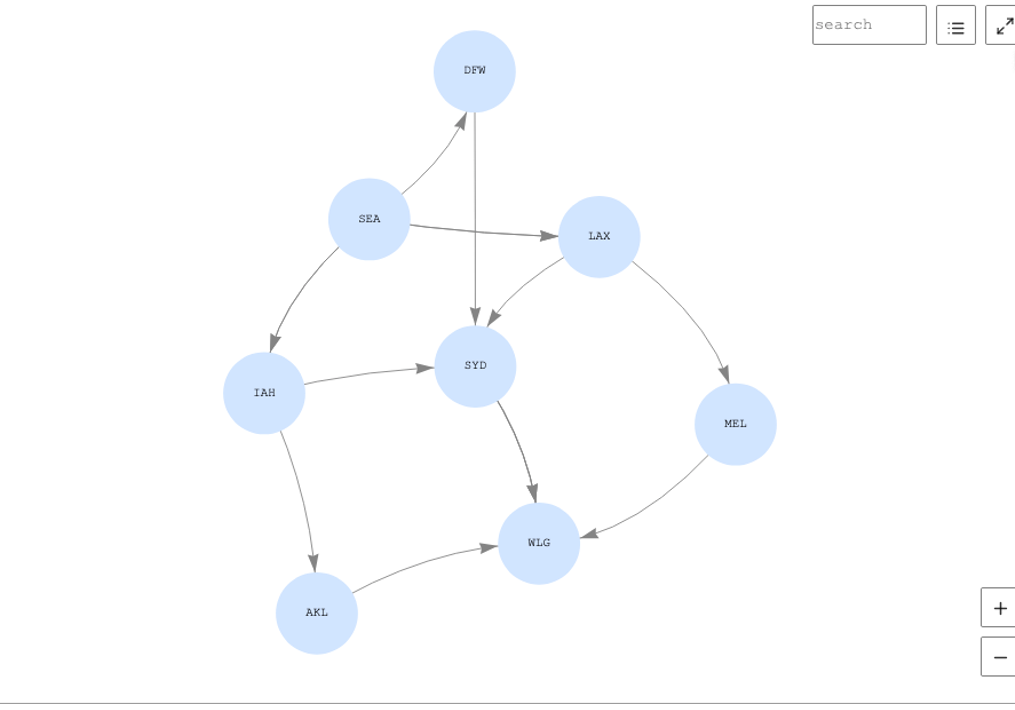
One of the questions in our use case was “What are the air routes from Seattle (SEA) to Wellington (WLG)?” In an RDBMS, this isn’t straightforward or efficient to determine because recursive self joins are usually needed. A graph traversal, however, is fast and intuitive. The following code shows a gremlin query and result, as a table, running in Neptune Workbench:

g.V().has('airport', 'airport_code', 'SEA') 
     .repeat(out().simplePath()) 
     .until(has('airport_code', 'WLG')) 
     .limit(5) 
     .path() 
     .by('airport_code') 

Neptune Workbench also allows visualization, and you can see the solution presented as a graph.

The other question we posed in part one of the series was, “What is the minimum number of stops required to fly from Seattle to Agra?” This is inefficient to answer in a relational model because an unknown number of self joins are required. The following Gremlin traversal can answer the question much more efficiently. Here we limit the maximum hops to five and the results to 10:

g.V().has('airport', 'airport_code', 'SEA') 
  .repeat(out('route').simplePath()) 
  .until(has('airport_code', 'AGR').or().loops().is(5)) 
  .has('airport_code', 'AGR') 
  .limit(10) 
  .path().by('airport_code') 

The results show that a minimum of three stops are required, all of them through Mumbai.

Summary

This series of posts discusses how to translate a relational data model to a graph data model. In this post, we designed a mapping from our relational data model to a labeled property graph model. In part three, we design an RDF model from our relational data model. We use the configuration file that defines the mapping in part four of the series.

If you have any questions, comments, or other feedback, share your thoughts on the Amazon Neptune Discussion Forums.

About the author

Chris Smith is a Principal Solutions Architect on the AWS Database Services Organization Customer Advisory Team focusing on Neptune. He works with customers to solve business problems using Amazon graph technologies. Semantic modeling, knowledge representation, and NLP are subjects of particular interest.